[CA6] Parallel Processors from Client to Cloud

(“이건 책 내용대로 말고 나름대로 묶어서 프린트 만들었다.”)

1. Introduction
2. Amdahl’s Law
3. Performance Scaling
4. Data Parallelism
   1. SIMD(Single-Instruction Multiple-Data)
   2. Vector Processors
5. Task/Thread-Level Parallelism
   1. Hardware Multithreading
   2. Multicores
   3. parallel Architectures
6. Introduction

Goal: Connecting multiple computers (i.e. 1 CPU or core) to get higher performance

Multicore microprocessors: Chips with multiple processors (cores)

Please distinguish between these two things:

• Job-level (process-level) parallelism

  High throughput for independent jobs

• Parallel processing program

  Single program run on multiple processors ~ Multithreading?

The goal of parallel programming

Making effective use of parallel hardware.

We need to get significant performance improvement, better than simply using a faster uniprocessor.

Difficulties (3)

• Partitioning - Our FOCUS!
• Coordination
• Communication Overhead

cf. The later two are similar. e.g. in somewhat called Partial processing, as the number of nodes get higher, the communication overhead increases (my guess: O(n^2)), and this gives discrepancies of the real-world performance and the ideal performance of parallel programming.  We learn the later two things in a senior's class, the Parallel Computing.

Amdahl’s Law

terms:

• serial portion == sequential portion (S)

  The non-paralizable part of the code. Antonym: Paralizible portion (P) of the code.

\[SpeedUp = \frac{1}{(1-P) + \frac{P}{n}}\]

• S = (1-P) : time portion of executing the serial portion in the original, non-paralized code.
• n: number of processor cores.

Amdahl’s Law:

• A theoretical basis by which the speedup of parallel computations can be estimated.
• The theoretical upper limit of speedup is limited by the serial portion of the code.

Example:

• Query: Let’s say that we have 100 processors, and we want to have x90 Speedups. What would be the required parallel portion P of the code?

• Answer: We want the following P that satisfies the Amdahl’s Law with n=100 and speedup=90: \(90 = \frac{1}{(1-P) + \frac{P}{100}}\) \(90*(100-99P) = 100\) Hence \(P = \frac{100 * 89}{99 * 90}\)

  Solving the generalized version, we get \(P = \frac{n * (r-1)}{(n-1) * r}\)

  Hence, P = 0.998877665544332

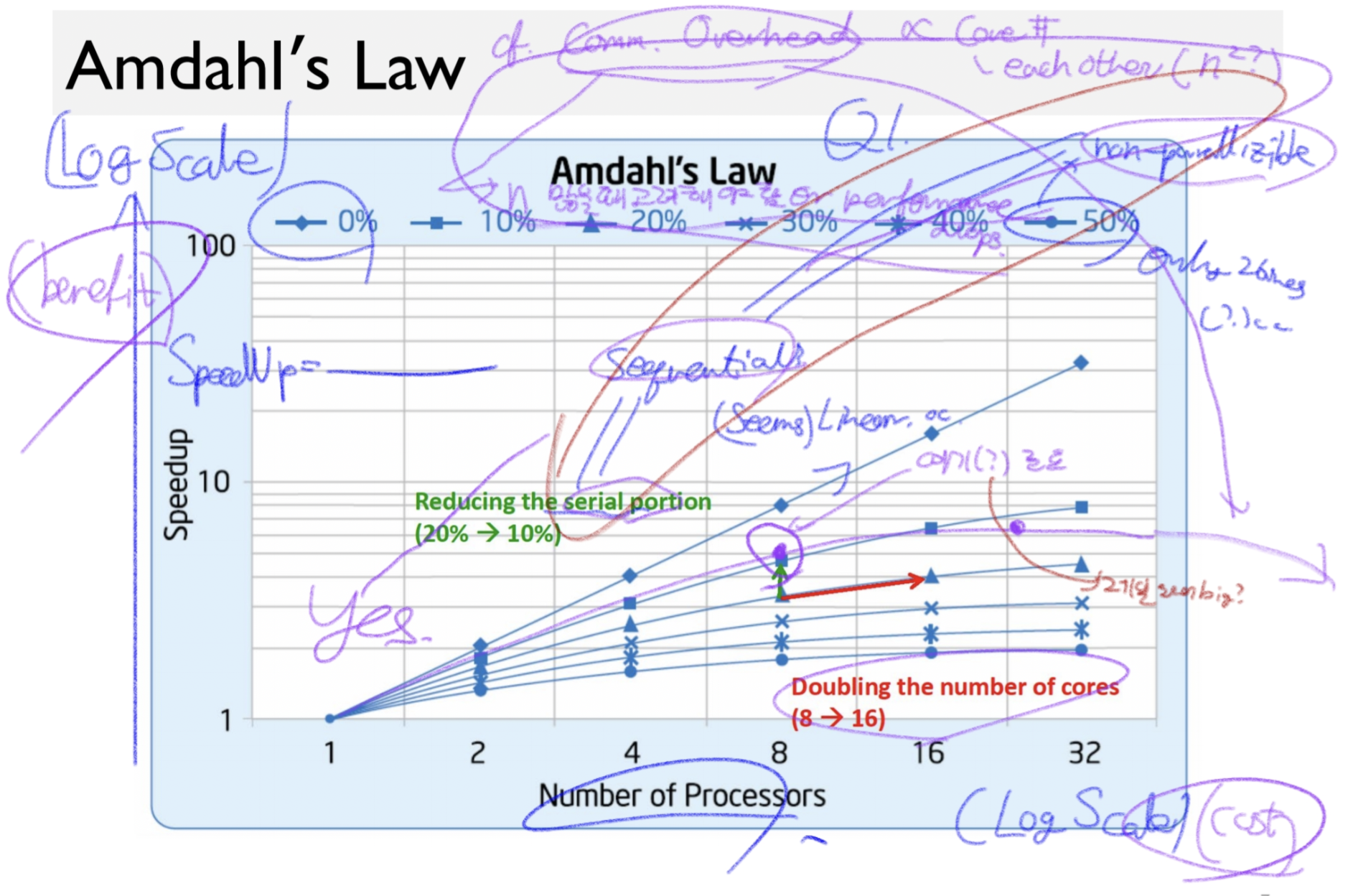
In this log cost - log benefit graph, consider the benefit per cost:

• In the both log-scaled graph, we would want the distance from the line y=x be the greatest.
• Find the point at which the tangent line’s slope is 1. That is the position we want in this graph.
• [N] Neither the peak nor the limit value is not what we want.
• [N] Graph being actually decresased after reaching a peak

Performance Scaling

Scaling Examples

• Workload: Sum of t scalars, and rt*rt matrix sum, n processors.
  • Assume only matrix sum is parallizable.
  • Assume load is balanced across processors. (: uniformly/equally partition the paralizable tasks, thereby giving linear speedup.)

Time:

• Single processor: \(t =\)

ㅇㅇ.

e.g.1. n = 1, 10, 100

(a, b): (Time/SpeedUp ratio (= Quiz starts at ))

n\rt	10	100
1	…	…
10	…	…
100	…	…

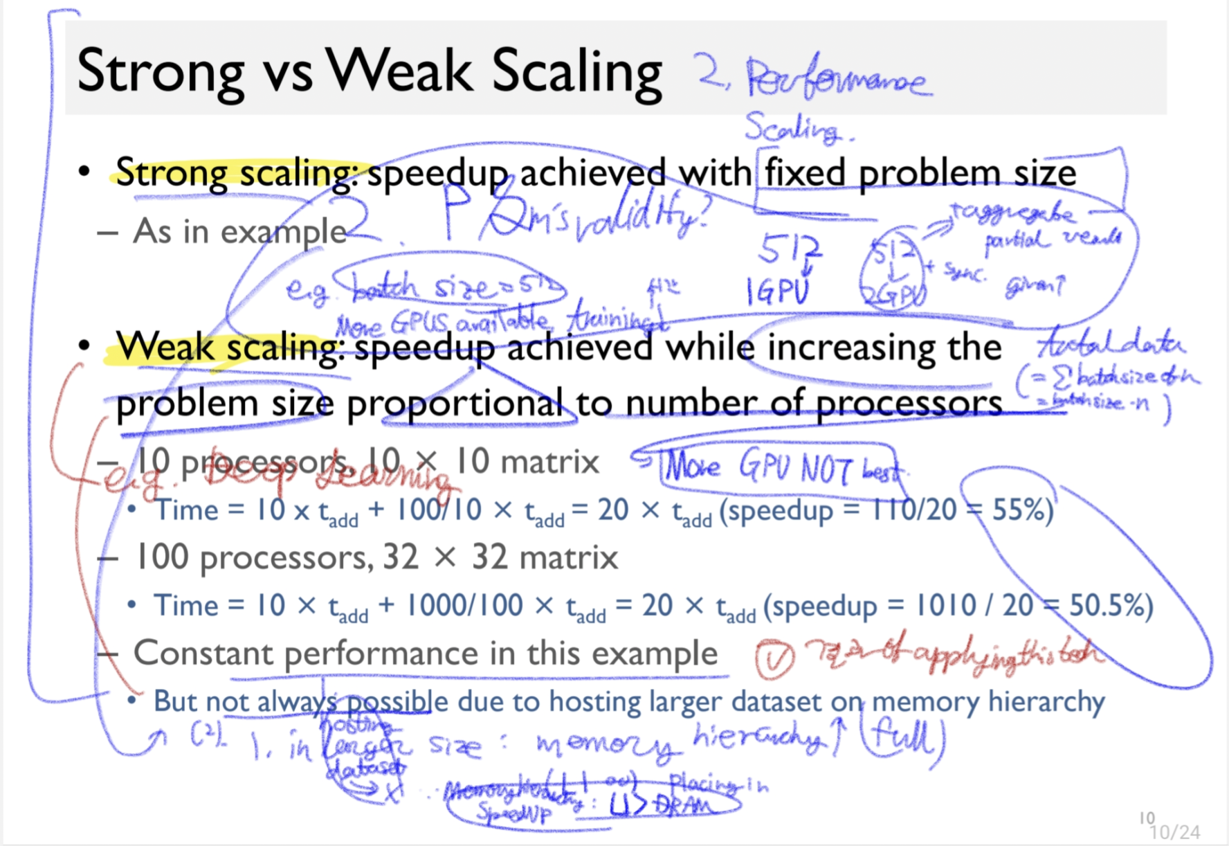
Strong and Weak Scaling

• Strong scaling: The speedup achieved with fixed problem size, as in the aformentioned e.g..
• Weak scaling: The speedup achieved with increasing the problem size in proportion to the number of processors. e.g. DL.

Intro to parallelism.

Types of parallelism:

• Instruction-Level Parallelism (learned in Ch.4, 5)
  • Pipelining, superscalar, speculation, branch prediction, out-of-order (OOO, O3), VLIW, …
• Data-Level Parallelism
  • SIMD extensions
  • Vector Architecture
• Task/Thread-Level Parallelism
  • Simultaneous Multithreading
  • Multicore Processors

Data Parallelism

An ILP concerns with “issue waste”s.

Vertical waste: The completely unfilled issue(box?) between two nonempty issues. (뇌피셜)

Horizontal wastes: The part of unfiled issue slots in a nonempty box. (뇌피셜)

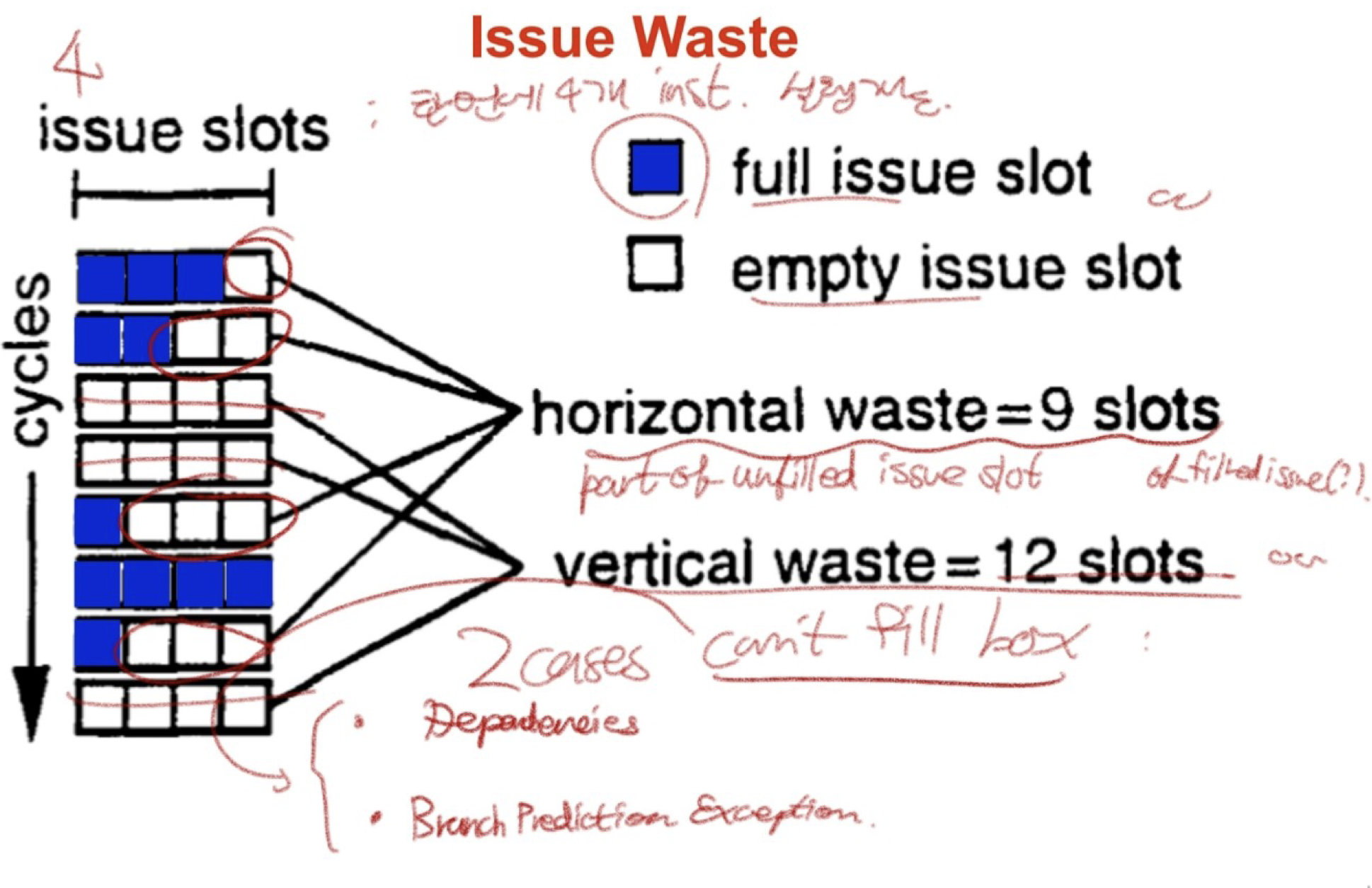
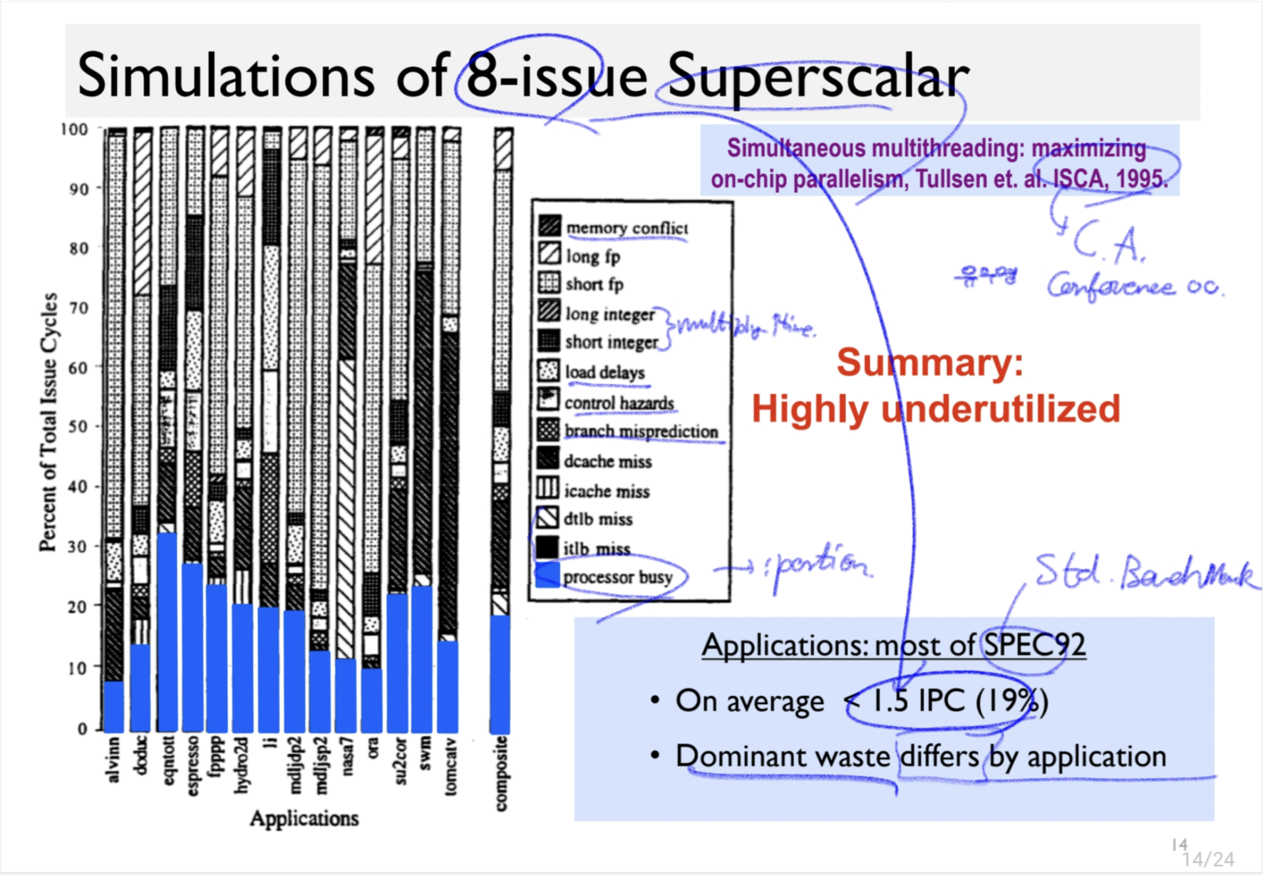
Some Sources of Wasted Issue Slots

• Memory Hierarchy
  • TLB miss
  • I cache miss
  • D cache miss
  • Load delays (L1 hits)
• Control Flow
  • Branch misprediction
• Instruction Stream
  • Instruction dependences
  • Memory conflict

What would be the parallelism granularity of this code here?

for(int i=0;i<1000;i++) {
  c[i] = a[i] + b[i];
}

an addition instruction? The professor said that that would be correct in case of MIMD.

The answer the professor said is the data. (probably in SIMD.)

So what the heck are MIMD and SIMD? Let’s take a closer look.

SIMD (Single-Instruction Multiple-Data)

SIMD vs. MIMD

Vector Processors

Task/Thread-Level Parallelism

Hardware Multithreading

“걍 coarse, fine-graining, SMT가 뭔지만 알라.”

• Fine-grain multithreading
  • Switch threads after each cycle.
  • Interleave instruction execution (: HDD 성능 높이기 위해 데이터가 서로 인접하지 않도록 배열하는 방식.)
  • If one thread stalls, others are executed.
• Coarse-grain multithreading
  • Only switch on long stall (e.g. L2-cache miss)
  • Simplifies hardware, but doesn’t hide short stalls. (e.g. data hazards.)

Simultaneous Multithreading (SMT)

• In multiple-issue dynamically scheduled processor,
  • Schedule instructions from multiple threads.
  • Instructions from independent threads execute when function units are available.
  • (cf. The dependencies within threads are handled by scheduling and register renaming.)
• Uses processor resources more effectively.
• e.g. Intel i7 HyperThreading
  • (2 threads, duplicated registers, shared function units and caches.)

Multithreading Examples

내가 볼 땐 이 그림이 완전완전 중요한듯.

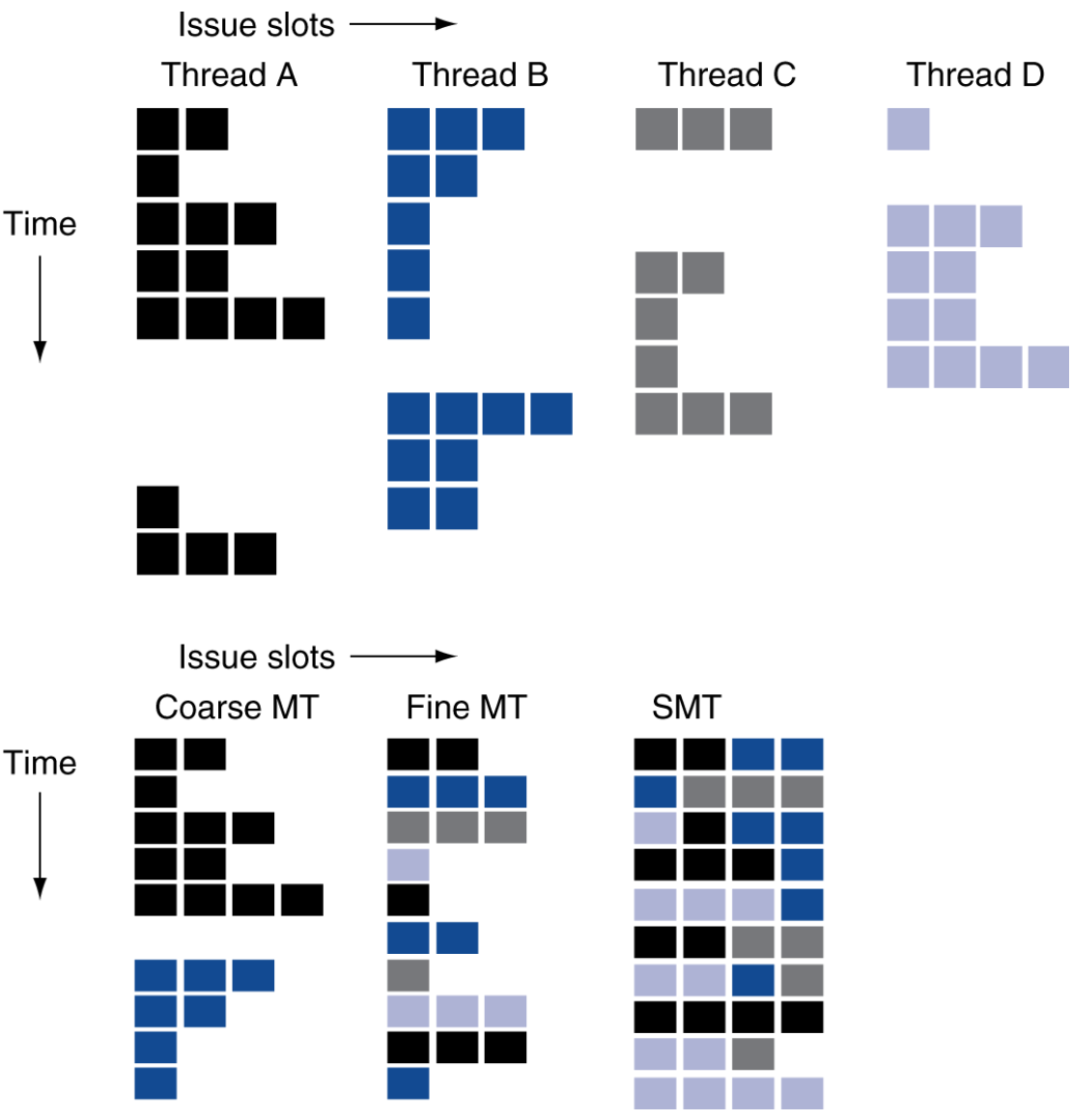
걍 Basic vs. SMT pipeline

…

Q. 저 그림의 경우

HW적으로 SMT가 더 복잡한 건 사실인데 그게 더 효율적이긴 하다.

Multicores

?

Parallel Architectures